Towards Model Predictive Control, Part 1

Why MPC?

Model predictive control is useful for problems for which reactive control methods (like PID) are insufficient. Insulin dynamics are one such problem; a purely reactive controller is prone to overshoot, because the action of the insulin happens after a long delay from its delivery. A good model predictive controller will account for this long delay to find an optimal control action. Most of the effective AP controllers are of this type.

Setting up a Model Predictive Controller

An MPC controller is formed by producing a set of state-space and input constraints from a plant model, determining a cost function which will incentivize good control, and optimizing the cost function across the space of controller inputs and modeled plant outputs. The optimal control value is found by finding the set of controller actions which results in the lowest cost over some finite horizon. The choices for modeling state and cost functions are constrained to those which are mathematically solvable.

We are using cvxpy to develop our controller.

We use the model developed by Van Heusden, et al as a simple LTI model for our controller. First, we define some constants:

T = 100
init_state = 250
p1 = 0.98
p2 = 0.965
g = -90 * (1 - p1) * (1 - p2) * (1 - p2)
u_TDI = 60

Here, T is the prediction horizon, in discrete samples, where each sample is ~5 mins. We will perform an optimization during every control step; so here, init state is the current state. p1, p2, and g are constants which describe the blood glucose dynamics. u_TDI is the subject-specific daily insulin.

Our simple model is described by

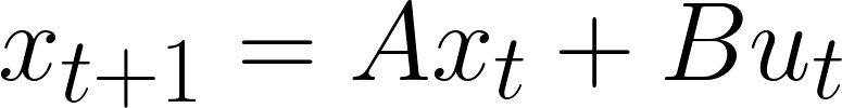
Where

And

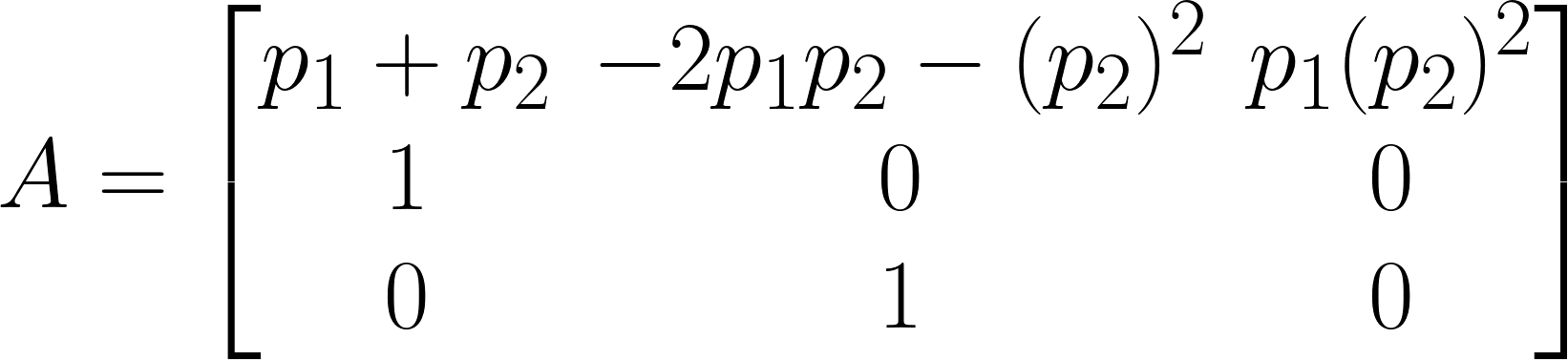
Thus, we have:

A = np.array([   
        [p1+2*p2, -2*p1*p2-p2*p2, p1*p2*p2],
        [1,0,0],
        [0,1,0]])
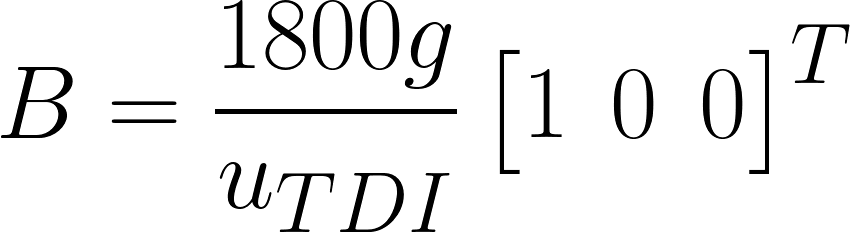
B = 1800 * g / u_TDI * np.array([[1],[0],[0]])

We define our variables as cvxpy variables, this way the solver can work with them:

x = cp.Variable((3, T+1))
u = cp.Variable((1, T))

The variables are 2-D arrays; 3 values of x are used to describe the state of the blood glucose at each step within the prediction horizon T – plus one additional step, to account for the control action at the last step within the control horizon. Thus x is an array with 3 rows and T+1 columns. u is an array with T columns, because we can only have a single control action for each step.

Then, we initialize the cost:

cost = 0

cvxpy takes constraints in the form of an array. We will populate the constraints using our model – the possible range of states can only be those that arise as the result of control actions based on our model.

constraints = []

We tell cvxpy how to build the array of values that our state variables and our control variables can possibly be, as well as the cost of each and the constraints placed on each. The cost function penalizes BG values that are far away from 100, as well as large controller actions. We also add a constraint of the maximum possible control action:

for t in range(T):
    cost += cp.sum_squares(x[:,t] - 100) + cp.sum_squares(u[:,t])
    constraints += [
        x[:,t+1] == A @ x[:,t] + B @ u[:,t],
        cp.norm_inf(u[:,t]) <= 1
    ]

Finally, we add one more constraint: that the value of the current blood sugar, at x[:,0] is equal to the current blood sugar:

constraints += [
    x[:,0] == init_state
]

We then tell the solver to minimize the cost across the space of all constraints and solve the optimization problem:

problem = cp.Problem(cp.Minimize(cost), constraints)
problem.solve(verbose=True)

We plot the results, and we can see that the controller has developed the optimal control strategy based on how it thinks the blood sugar will behave in the space of all possible control inputs according to our model. So long as our model forms a reasonable approximation for the blood glucose response, our controller has charted an optimal future course.

Top is the blood glucose response and the bottom is the controller response.

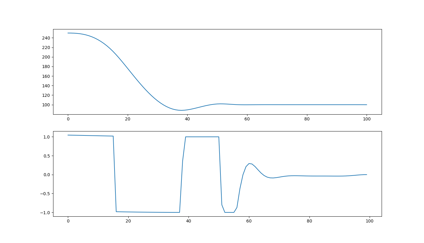
We would then take the first step, u[:,0], as our next controller action, and repeat the process at the next control step.

Issues

There are a couple of issues with this, though. First, this allows for negative control actions, which would be equivalent to delivering negative amounts of insulin. Secondly, the cost function penalizes low values the same as high values and only has a single optimal value (100). Finally, the constraints placed on the controller response are relatively minor; we have only specified that it cannot exceed 1 unit per time-step, which is not a hard enough constraint as the total insulin delivered could easily surpass a safe maximum amount.

However, this is a good first step for a controller.