[1]:
import os, pathlib
os.chdir(pathlib.Path(globals()['_dh'][0]).parent)
Animation + Plot Example#
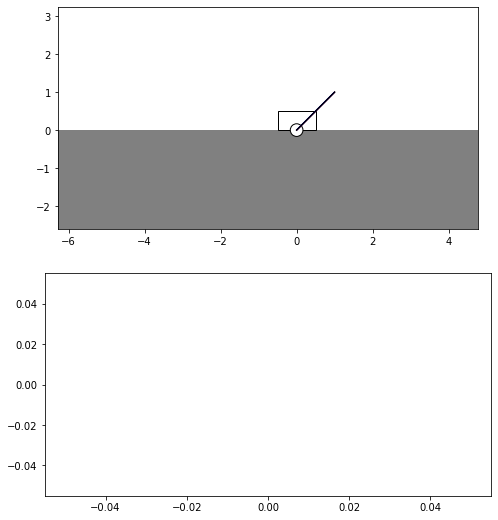
pendsim includes the ability to generate animated plots alongside the animation of the simulation. This is helpful when visualizing specific pendulum states along with the animation. For this example, we will create a PID controller with an Unscented Kalman Filter, and then visualize the measured state with the filtered measurements to see how this functionality might be used.
Arrange imports
[2]:
from pendsim import sim, controller, viz
import numpy as np
import matplotlib.pyplot as plt
Create a pendulum with a 2kg cart, 1kg mass, and 2-meter length. The initial state is given by the initial_state arg. The state array is \(\textbf{x}=[x, \dot{x}, \theta, \dot{\theta}]\) So in this case the pendulum starts slightly tipped over: \(\theta = 0.1\).
[3]:
pend = sim.Pendulum(
    2.0,
    1.0,
    2,0,
    initial_state = np.array([0.0, 0.0, 0.1, 0.0])
)
Create a PID controller with gains kp, ki, kd. For this example, we use the PID controller with an unscented Kalman Filter, so that we can visualize in real time the filter’s performance at estimating the state (given as noisy, discrete points).
PID_UKF takes one additional argument, var_t, which is the backwards window, in seconds, over which to measure the variance in the state. So, at every point, we look backward over a period of 0.2s, measure the variance, and then use the variance to estimate the true state from noise via Unscented Kalman Filtering. For more details about Unscented Kalman Filtering, see https://groups.seas.harvard.edu/courses/cs281/papers/unscented.pdf.
dt is the timestep of the simulation. Because the simulation solves an I.V.P (Initial Value Problem) at every timestep to determine the simulated pendulum’s position, dt can be large without introducing numerical errors. The controller’s action is taken at intervals of dt and held constant throughout the interval. We must pass the same value for dt to the controller as is used by the simulation.
So, because we are creating the controller here, dt is specified here.
[4]:
kp, ki, kd = 20.0, 0.0, 2.0

dt = 0.02

cont = controller.PID_UKF(
    # PID gains
    (kp, ki, kd),
    pend,
    dt,
    # var_t
    0.2
)
Create a simulation object with a timestep dt, run time t_final, and an 20N impulse force that peaks at t= 2seconds
[5]:
t_final = 12.0
def force(t):
    return 20 * np.exp( -((t-2.0)/0.1)**2 )

noise_scale = np.array([0.1,0.1,0.1,0.1])

simu = sim.Simulation(dt, t_final, force, noise_scale=noise_scale)
Run the simulation with the pendulum and controller we created and store the simulation results into results
[6]:
results = simu.simulate(pend, cont)
100%|██████████| 600/600 [00:02<00:00, 213.01it/s]
We can see the available states by printing results.columns.
The pltdata dict stores all of the parameters for generating the animated plot. There are two types of animated plots: line plots and scatter plots. For line plots, we must supply the linestyle argument; for both types of plot, we must supply label, color, and plotpoints args. The key of pltdata is the same as the column contained in results that we want to measure and display in the animation.
In this example, we display the “true state” theta, given by ('state', 't'); the state actually measured by the controller, given by ('measured state', 't'); and the estimated state, given by ('est','t'). Note that the ('est','t') column is one that is stored directly by the controller’s policy.
[7]:
print(results.columns)
pltdata = {
    ('state', 't') : {
        # The plot type, line or scatter
        'type' : 'line',
        # The label generated in the plot window
        'label' : 'true theta',
        # The style of the line, e.g. '--' produces a dotted line
        'linestyle' : '-',
        # The line color
        'color' : 'r',
        # The number of plot points to draw on the canvas
        'plotpoints' : 50,
    },
    ('measured state', 't') : {
        # scatter types don't need `linestyle` kwarg.
        'type' : 'scatter',
        'label' : 'measured theta',
        'color' : 'k',
        'plotpoints' : 50,
    },
    ('est', 't') : {
        'type' : 'line',
        'label' : 'estimated theta',
        'linestyle':'--',
        'color' : 'g',
        'plotpoints': 50,
    }
}
MultiIndex([(         'state',              'x'),
            (         'state',             'xd'),
            (         'state',              't'),
            (         'state',             'td'),
            ('measured state',              'x'),
            ('measured state',             'xd'),
            ('measured state',              't'),
            ('measured state',             'td'),
            ('noise variance',              'x'),
            ('noise variance',             'xd'),
            ('noise variance',              't'),
            ('noise variance',             'td'),
            (           'res',              'x'),
            (           'res',             'xd'),
            (           'res',              't'),
            (           'res',             'td'),
            (           'est',              'x'),
            (           'est',             'xd'),
            (           'est',              't'),
            (           'est',             'td'),
            (        'energy',        'kinetic'),
            (        'energy',      'potential'),
            (        'energy',          'total'),
            (        'forces',         'forces'),
            ('control action', 'control action'),
            (        'forces',            'pRx'),
            (        'forces',            'pRy'),
            (        'forces',             'pG'),
            (        'forces',            'cRy'),
            (        'forces',            'cRx'),
            (        'forces',             'cG'),
            (        'forces',             'cN')],
           )
Make an animation of the simulation. Make sure to bind the result of visu.animate() to a variable, because that is required in order to ensure that the animation will actually run.
[8]:
visu = viz.Visualizer(results, pend, dt, speed=1)
ani = visu.animate(pltdata=pltdata)

In web-based notebooks, animations may not display correctly with just the matplotlib plots. It may be necessary to run the following cell to render and view an HTML5 video of the animation.
[9]:
from IPython.display import HTML
HTML(ani.to_html5_video())
[9]: